Comparing Cox and flexible parametric models
Table of Contents
The code used in this tutorial is available here.
Introduction
This is a companion to the tutorial on standardised survival curves, where we compare compare survival between males and females diagnosed with melanoma after fitting a flexible parametric survival model. This companion is aimed at readers familiar with the Cox model, but not flexible parametric models. The aim is to illustrate that flexible parametric models are conceptually very similar to the Cox model (and provide similar estimates) but have benefits compared to the Cox model if one is interested in estimating quantities other than hazard ratios.
Paul Lambert has also written a tutorial showing the similarities between Cox model and flexible parametric proportional hazards models, but using a different example.
Comparing PH models
Here we fit proportional hazards models and show that the estimated hazard ratios are very similar. I am yet to see an example of proportional hazards models where they are markedly different. I’ve omitted the output from the model fitting and just shown the table of parameter estimates, but the code is available to reproduce the complete output.
. use https://pauldickman.com/data/melanoma.dta if stage>0, clear
(Skin melanoma, diagnosed 1975-94, follow-up to 1995)

. // cause-specific survival (status==1 is death due to melanoma)
. stset surv_mm, fail(status==1) scale(12) exit(time 120)

. // create dummy variables for modelling
. generate male=(sex==1)

. // spline variables for year of diagnosis
. rcsgen yydx, df(3) gen(yearspl) orthog

. stpm2 i.male yearspl* i.agegrp, scale(h) df(5) eform
. estimates store adj1

. stpm2 i.male yearspl* i.agegrp i.stage i.subsite, scale(h) df(5) eform
. estimates store adj2

. stcox i.male yearspl* i.agegrp
. estimates store adj1_cox

. stcox i.male yearspl* i.agegrp i.stage i.subsite
. estimates store adj2_cox

. estimates table adj1 adj1_cox adj2 adj2_cox, eform equations(1) ///
>   b(%9.6f) modelwidth(12) keep(i.male i.agegrp i.stage i.subsite)

--------------------------------------------------------------------------
    Variable |     adj1         adj1_cox         adj2         adj2_cox
-------------+------------------------------------------------------------
        male |
          0  |       (base)         (base)         (base)         (base)
          1  |     1.787024       1.782951       1.335592       1.334913
             |
      agegrp |
       0-44  |       (base)         (base)         (base)         (base)
      45-59  |     1.352939       1.351643       1.284287       1.282252
      60-74  |     1.796602       1.792671       1.645531       1.642131
        75+  |     2.860405       2.840446       2.610964       2.592047
             |
       stage |
  Localised  |                                     (base)         (base)
   Regional  |                                   4.700280       4.676851
    Distant  |                                  13.501379      13.271929
             |
     subsite |
Head and ..  |                                     (base)         (base)
      Trunk  |                                   1.410452       1.404551
      Limbs  |                                   1.031511       1.028769
Multiple ..  |                                   1.360867       1.352698
--------------------------------------------------------------------------
You may ask, if the parameter estimates are the same then why not just use the well-known Cox model? This is a reasonable question, and if all you want are hazard ratios then the Cox model serves that purpose. However, there are quantities of interest other than the hazard ratio and these are much easier to obtain after fitting a flexible parametric model. Standardised survival curves are one such example.
Hazard ratios are easier to interpret if one assumes they are constant over time (i.e., an assumption of proportional hazards), an assumption that is not always appropriate. For example, Andreassen and colleagues studied sex differences in bladder cancer survival and presented the following graph showing that the sex effect was not constant over follow-up.
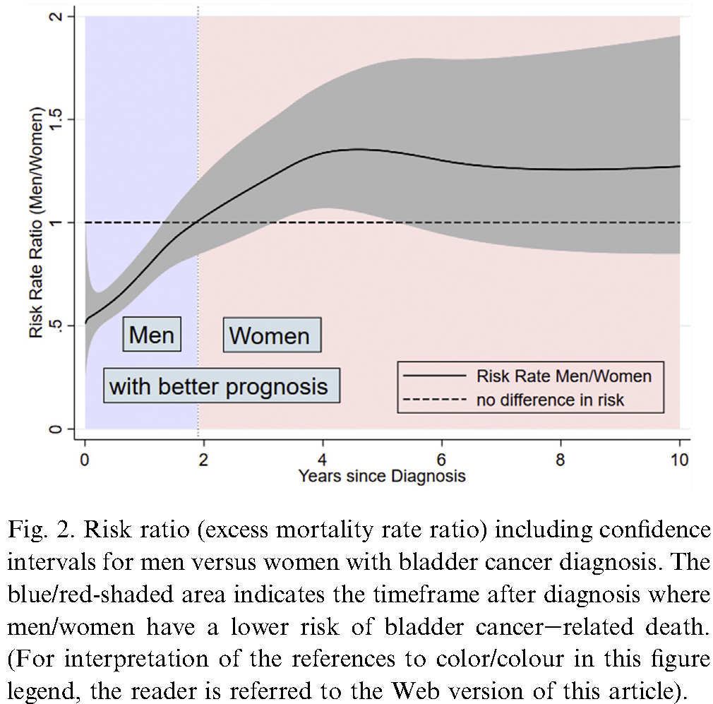
Such graphs are very easy to obtain after fitting a flexible parametric survival model (see example below). The interpetation of hazard ratios has been questioned (see Miguel Hernán’s comments on the hazards of hazard ratios), but making an assumption they are constant over time is especially problematic. Hernán argues one should estimate standardised survival curves of the type we describe in our tutorial.
Graphing the HR as a function of time
Here I illustrate how to obtain a graph of the time-varying hazard ratio for the melanoma data similar to that shown above for bladder cancer. We first fit a flexible parametric model allowing the effect of sex to be time-varying (i.e., non-proportional hazards).
. stpm2 male yearspl* i.agegrp, scale(h) df(5) eform tvc(male) dftvc(3)

Log likelihood = -5185.8573                     Number of obs     =      6,144

------------------------------------------------------------------------------
             |     exp(b)   Std. Err.      z    P>|z|     [95% Conf. Interval]
-------------+----------------------------------------------------------------
xb           |
        male |   1.783504   .0957656    10.78   0.000     1.605346    1.981433
    yearspl1 |   .8657204   .0244292    -5.11   0.000       .81914    .9149495
    yearspl2 |   .9097286   .0247784    -3.47   0.001     .8624373     .959613
    yearspl3 |   .9726465    .026693    -1.01   0.312     .9217113    1.026396
             |
      agegrp |
       0-44  |          1  (base)
      45-59  |   1.352094   .0992726     4.11   0.000     1.170875    1.561361
      60-74  |   1.794815   .1277099     8.22   0.000     1.561179    2.063417
        75+  |   2.859922   .2371981    12.67   0.000     2.430842    3.364742
             |
       _rcs1 |   2.260808    .068249    27.02   0.000     2.130922     2.39861
       _rcs2 |   1.133291   .0277438     5.11   0.000     1.080198    1.188993
       _rcs3 |   1.074457   .0148835     5.18   0.000     1.045678    1.104027
       _rcs4 |   1.018815   .0081562     2.33   0.020     1.002954    1.034927
       _rcs5 |   1.003467   .0043966     0.79   0.430     .9948868    1.012121
  _rcs_male1 |   1.016583   .0402922     0.41   0.678     .9406016    1.098703
  _rcs_male2 |    1.04943   .0350462     1.44   0.149     .9829408    1.120417
  _rcs_male3 |   1.012232   .0185113     0.66   0.506      .976593    1.049172
       _cons |    .099029   .0065442   -34.99   0.000     .0869986     .112723
------------------------------------------------------------------------------
Note: Estimates are transformed only in the first equation.
I have chosen to model the effect of year of diagnosis using a restricted cubic spline. I created the 3 spline basis vectors (yearspl1-yearspl3) using the rcsgen command (code shown above); 3 degrees of freedom corresponds to 2 internal knots and 2 boundary knots (see the help for rcsgen).
Fitting a flexible parametric survival model involves modelling the baseline cumulative hazard using restricted cubic splines. I specified the df(5) option to stpm2, which results in the spline basis variables _rcs1 to _rcs5 being created and included in the linear predictor. The time-varying effect of sex is modelled using a restricted cubic spline with 3 df (the dftvc(3) option); the spline basis variables _rcs_male1 to _rcs_male1 are also created by stpm2. The estimated hazard ratios (exp(b)) for age group in the table above have the usual interpretation, but none of the other hazard ratios in the table above has a simple interpretation. The hazard ratio for male does not have a simple interpretation because we have modelled a time-varying effect of sex.
We now create a temporary time variable and use the predict command to save the predicted hazard ratio (males to females) to the new variable hr.
. range temptime 0 10 51
(6,093 missing values generated)

. predict hr, hrnumerator(male 1) ci timevar(temptime)

. twoway (rarea hr_lci hr_uci temptime, color(red%25)) ///
>        (line hr temptime, sort lcolor(red)) ///
>       , legend(off) ysize(8) xsize(11) ///
>        ytitle("Hazard ratio (male/female)") name("hr", replace) ///
>        xtitle("Years since diagnosis")

Do we need to allow for a time-varying effect of sex?
The answer to this question depends on both subject-matter considerations (e.g., clinical significance) and statistical significance. I support the view that the interpretation of scientific studies should be based on more than statistical significance (see the March 2019 commentary Scientists rise up against statistical significance in Nature).
If we refit the model assuming proportional hazards for sex (i.e., removing tvc(male) dftvc(3)), the estimated hazard ratio is 1.787. Assuming our model is appropriate for confounding control (which it is not given we haven’t adjusted for stage and subsite), the question reduces to “are we willing to assume the HR is 1.79 throughout the follow-up or does it vary in the manner shown in the figure above?”. When intepreting ratio measures, it is important to be aware of the underlying absolute risks, in this case the two hazard functions. We can easily obtain the empirical hazards as follows.
. sts graph, hazard by(sex) kernel(epan2) name(h, replace)

We see that the underlying hazards are higest between diagnosis and 4 years, so we should focus on this period. The hazards are very low after 6 years so we should not place too much weight on the HR for this period. Our question therefore reduces to “is it clinically or scientifically important to consider that the estimated hazard ratio varies between 1.7 and 1.9 (or from 1.6 to 2.0 if one is conservative)?”. I suggest the answer is probably no.
We can also test statistical significance, but should be aware that our test may not be powerful to detect clinically meaningful differences or (if we have a large study) differences that are not clinically important may be statistically significant. I chose to use 3 parameters to model the time-varying effect of sex. We could test statistical significance using a likelihood ratio test (the lrtest command), but I’ll use a Wald test since it requires just one command and precludes having to refit the models.
. testparm _rcs_male*

 ( 1)  [xb]_rcs_male1 = 0
 ( 2)  [xb]_rcs_male2 = 0
 ( 3)  [xb]_rcs_male3 = 0

           chi2(  3) =    3.90
         Prob > chi2 =    0.2723
There is no evidence of a statistically significant time-varying effect of sex. If the time-varying effect of sex could be adequately captured with just 2 df then we would have a more powerful test, but parameterising the test based on the observed data is not good science. Either way, it’s still not statistically significant (output not shown). Using just 1 df would not capture the form of the time-varying effect.
In summary, an assumption of proportional hazards for the effect of sex appears reasonable for the melanoma data. For the bladder cancer example, however, there is a much stronger and clinically important time-dependent effect of sex. For the bladder cancer example, however, one should be aware that mortality is highest in the period up to 3 years post diagnosis so focus should be on that period.
Paul Dickman
Professor of Biostatistics
Biostatistician working with register-based cancer epidemiology.