Illustration of the strs algorithm for estimating relative survival
The code used in this tutorial, along with links to the data, is available here.
This page illustrates the algorithm used by strs for estimating relative survival using the Ederer II approach. The basic algorithm is as follows.
- Split person-time into life-table intervals
- Generate attained (updated) age and calendar year
- Merge with popmort file to get the expected probabilities
- Collapse to one observation for each life table interval (summing deaths and censoring and averaging expected survival)
- Calculate interval-specific survival
- Multiply interval-specific estimates to get cumulative estimates
The code on this page assumes annual life table intervals, whereas strs allows intervals of any width.
The following block shows steps 1 and 2. We use the scale(12) option to stset so that the time units are in years (surv_mm is survival time in years) and then use stsplit to splity time into yearly intervals. We then generate variables for updated (interval-specific) age and calendar year.
. use http://pauldickman.com/data/melanoma if stage==1 , clear
.
. stset surv_mm, fail(status==1 2) id(id) scale(12)

. // Split into annual intervals
. stsplit start, at(0(1)25)
(35,974 observations (episodes) created)

.
. // Generate attained (updated) age and calendar year
. gen _age=floor(age+_t0)

. gen _year=floor(yydx+_t0)

.
. // Merge with popmort file to get the expected probabilities of death
. merge m:1 sex _age _year using http://pauldickman.com/data/popmort, keep(match master) nogenerate keepusing(prob)

    Result                           # of obs.
    -----------------------------------------
    not matched                             0
    matched                            41,292
    -----------------------------------------

. sort id start
Below we see the resulting data for the first two patients after splitting and merging. We see that age at diagnosis (age) and year of diagnosis (yydx) are constant for each interval whereas attained age (_age) and updated year of diagnosis (_year) are updated to reflect the values current for the interval.
. list id _t0 _t _d age _age yydx _year prob if inlist(id,1,2), sepby(id) noobs

  +----------------------------------------------------------------+
  | id   _t0          _t   _d   age   _age   yydx   _year     prob |
  |----------------------------------------------------------------|
  |  1     0           1    0    81     81   1981    1981   .91931 |
  |  1     1           2    0    81     82   1981    1982   .90841 |
  |  1     2   2.2083333    1    81     83   1981    1983    .9012 |
  |----------------------------------------------------------------|
  |  2     0           1    0    75     75   1975    1975    .9459 |
  |  2     1           2    0    75     76   1975    1976    .9488 |
  |  2     2           3    0    75     77   1975    1977   .94384 |
  |  2     3           4    0    75     78   1975    1978   .93809 |
  |  2     4       4.625    1    75     79   1975    1979   .92965 |
  +----------------------------------------------------------------+
Below we see the resulting data for the first two patients after splitting and merging. We see that age at diagnosis (age) and year of diagnosis (yydx) are constant for each interval whereas attained age (_age) and updated year of diagnosis (_year) are updated to reflect the values current for the interval.
We now generate an indicator for censored during the interval (individuals who did not survive the last interval but did not die). We then collapse the data to obtain one observation per life table interval. When collapsing, we sum the number of events and censoring but average the expected survival. We then generate the other life table quantities.
. // generate an indicator for censored during the interval
. bysort id : gen w = (_d[_N]==0 & _n==_N & (_t-_t0)!=1)

. // collapse to get one observation for each life table interval
. collapse (sum) d=_d w (count) n=_d (mean) p_star=prob, by(start)

. // effective number at risk
. gen n_prime=n-w/2

. // interval-specific observed survival
. gen p=1-d/n_prime

. // interval-specific relative survival
. gen r=p/p_star

. // multiply the interval-specific probabilities to get the cumulative probabilities
. // we use a*b = exp(ln(a)+ln(b)) since Stata can sum across observation but not multiply
. gen cp_e2=exp(sum(ln(p_star)))

. gen cp=exp(sum(ln(p)))

. gen cr_e2=exp(sum(ln(r)))
We now have our life table, and can list a table of estimates.
. list start n d w p p_star r cp cp_e2 cr_e2
     +--------------------------------------------------------------------------------+
     | start      n     d     w        p   p_star        r       cp    cp_e2    cr_e2 |
     |--------------------------------------------------------------------------------|
  1. |     0   5318   151     1   0.9716   0.9768   0.9947   0.9716   0.9768   0.9947 |
  2. |     1   5166   329   299   0.9344   0.9763   0.9571   0.9079   0.9537   0.9519 |
  3. |     2   4538   287   296   0.9346   0.9767   0.9569   0.8485   0.9315   0.9109 |
  4. |     3   3955   211   271   0.9448   0.9771   0.9669   0.8017   0.9102   0.8808 |
  5. |     4   3473   166   246   0.9504   0.9775   0.9723   0.7619   0.8897   0.8564 |
     |--------------------------------------------------------------------------------|
  6. |     5   3061   138   240   0.9531   0.9775   0.9751   0.7262   0.8696   0.8350 |
  7. |     6   2683   105   218   0.9592   0.9772   0.9815   0.6966   0.8499   0.8196 |
  8. |     7   2360    75   253   0.9664   0.9766   0.9896   0.6732   0.8299   0.8111 |
  9. |     8   2032    68   241   0.9644   0.9756   0.9885   0.6492   0.8097   0.8018 |
 10. |     9   1723    50   209   0.9691   0.9756   0.9933   0.6292   0.7900   0.7964 |
     |--------------------------------------------------------------------------------|
 11. |    10   1464    55   160   0.9603   0.9752   0.9847   0.6042   0.7704   0.7843 |
 12. |    11   1249    49   157   0.9581   0.9754   0.9823   0.5789   0.7514   0.7704 |
 13. |    12   1043    21   142   0.9784   0.9743   1.0042   0.5664   0.7321   0.7736 |
 14. |    13    880    22   168   0.9724   0.9728   0.9995   0.5507   0.7122   0.7732 |
 15. |    14    690    20   136   0.9678   0.9727   0.9950   0.5330   0.6928   0.7694 |
     |--------------------------------------------------------------------------------|
 16. |    15    534    15    97   0.9691   0.9728   0.9962   0.5165   0.6740   0.7664 |
 17. |    16    422    14   102   0.9623   0.9723   0.9897   0.4970   0.6553   0.7585 |
 18. |    17    306     7    91   0.9731   0.9718   1.0014   0.4837   0.6368   0.7596 |
 19. |    18    208     5    77   0.9705   0.9700   1.0005   0.4694   0.6177   0.7599 |
 20. |    19    126     6    59   0.9378   0.9655   0.9714   0.4402   0.5964   0.7382 |
     |--------------------------------------------------------------------------------|
 21. |    20     61     1    60   0.9677   0.9698   0.9979   0.4260   0.5784   0.7366 |
     +--------------------------------------------------------------------------------+
Our estimates are identical to those returned by strs.
. // We get the same results using strs
. use http://pauldickman.com/data/melanoma if stage==1 , clear
. stset surv_mm, fail(status==1 2) id(id) scale(12)
. strs using http://pauldickman.com/data/popmort, br(0(1)25) mergeby(_year sex _age)

No late entry detected - p is estimated using the actuarial method

  +------------------------------------------------------------------------------------------------------------+
  | start   end      n     d     w        p   p_star        r       cp    cp_e2    cr_e2   lo_cr_e2   hi_cr_e2 |
  |------------------------------------------------------------------------------------------------------------|
  |     0     1   5318   151     1   0.9716   0.9768   0.9947   0.9716   0.9768   0.9947     0.9897     0.9989 |
  |     1     2   5166   329   299   0.9344   0.9763   0.9571   0.9079   0.9537   0.9519     0.9434     0.9599 |
  |     2     3   4538   287   296   0.9346   0.9767   0.9569   0.8485   0.9315   0.9109     0.9000     0.9212 |
  |     3     4   3955   211   271   0.9448   0.9771   0.9669   0.8017   0.9102   0.8808     0.8682     0.8928 |
  |     4     5   3473   166   246   0.9504   0.9775   0.9723   0.7619   0.8897   0.8564     0.8424     0.8698 |
  |------------------------------------------------------------------------------------------------------------|
  |     5     6   3061   138   240   0.9531   0.9775   0.9751   0.7262   0.8696   0.8350     0.8198     0.8497 |
  |     6     7   2683   105   218   0.9592   0.9772   0.9815   0.6966   0.8499   0.8196     0.8033     0.8354 |
  |     7     8   2360    75   253   0.9664   0.9766   0.9896   0.6732   0.8299   0.8111     0.7938     0.8279 |
  |     8     9   2032    68   241   0.9644   0.9756   0.9885   0.6492   0.8097   0.8018     0.7833     0.8197 |
  |     9    10   1723    50   209   0.9691   0.9756   0.9933   0.6292   0.7900   0.7964     0.7768     0.8155 |
  |------------------------------------------------------------------------------------------------------------|
  |    10    11   1464    55   160   0.9603   0.9752   0.9847   0.6042   0.7704   0.7843     0.7631     0.8048 |
  |    11    12   1249    49   157   0.9581   0.9754   0.9823   0.5789   0.7514   0.7704     0.7476     0.7926 |
  |    12    13   1043    21   142   0.9784   0.9743   1.0042   0.5664   0.7321   0.7736     0.7496     0.7970 |
  |    13    14    880    22   168   0.9724   0.9728   0.9995   0.5507   0.7122   0.7732     0.7476     0.7983 |
  |    14    15    690    20   136   0.9678   0.9727   0.9950   0.5330   0.6928   0.7694     0.7415     0.7966 |
  |------------------------------------------------------------------------------------------------------------|
  |    15    16    534    15    97   0.9691   0.9728   0.9962   0.5165   0.6740   0.7664     0.7361     0.7961 |
  |    16    17    422    14   102   0.9623   0.9723   0.9897   0.4970   0.6553   0.7585     0.7248     0.7916 |
  |    17    18    306     7    91   0.9731   0.9718   1.0014   0.4837   0.6368   0.7596     0.7225     0.7960 |
  |    18    19    208     5    77   0.9705   0.9700   1.0005   0.4694   0.6177   0.7599     0.7177     0.8014 |
  |    19    20    126     6    59   0.9378   0.9655   0.9714   0.4402   0.5964   0.7382     0.6822     0.7932 |
  |------------------------------------------------------------------------------------------------------------|
  |    20    21     61     1    60   0.9677   0.9698   0.9979   0.4260   0.5784   0.7366     0.6632     0.8088 |
  +------------------------------------------------------------------------------------------------------------+
Actuarial versus hazard transformation approach
The estimation approach described above is known as the actuarial or life table approach. This approach is used by strs when there is no late entry (i.e., all patients are followed up from time zero). When there is late entry, as in period analysis, strs uses a different approach, the so-called hazard transformation approach. The hazard transformation approach is always used if the ht option is specified.
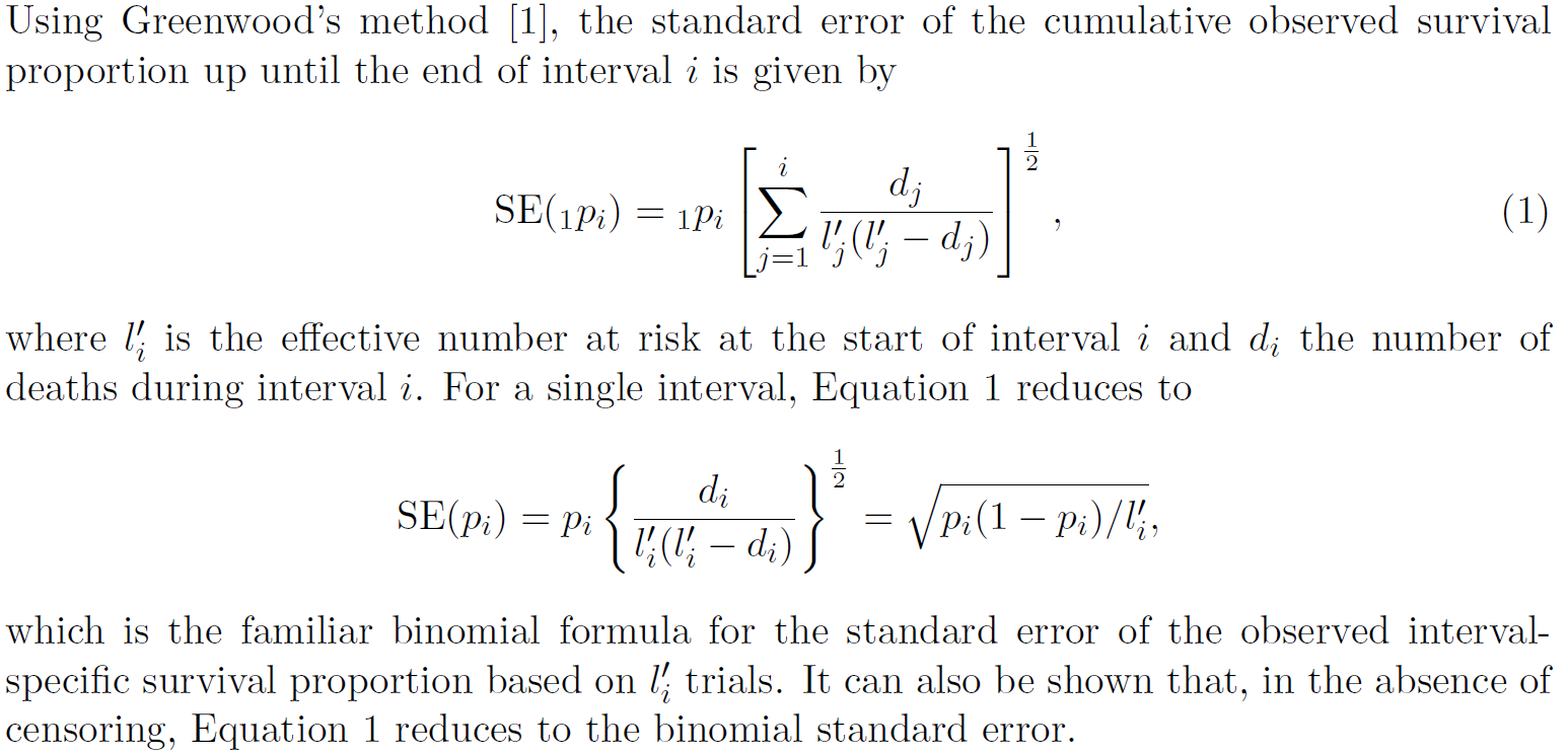
The actuarial estimator for the interval-specific observed survival for interval $i$ is
$$ p_i = (1-d_i/l’_i) $$
where $d_i$ is the number if deaths in the interval and $l’_i=1-w_i/2$ is the “effective number at risk” ($w_i$ is the number censored during the interval).
An alternative approach is to use the relationship that the survivor function is equal to the exponential of the negative of the cumulative hazard ($S=\exp(-\Lambda)$). We can estimate the average hazard for the interval as $\lambda_i=d_i/y_i$ where $d_i$ is the number of deaths and $y_i$ the person-time at risk in the interval. If the hazard is assumed to be constant at this value during the interval then the cumulative hazard for the interval is $\Lambda_i=k_i \times d_i/y_i$ where $k_i$ is the width of the interval. Our estimate of the interval-specific observed survival is therefore
$$ p_i = \exp(k_i \times -d_i/y_i) $$
Since this approach assumes the hazard is constant within the interval, it is sensitive to the choice of interval length, unlike the actuarial approach which gives the same estimates of cumulative observed survival independent of the choice of intervals.
Standard errors and confidence intervals
Actuarial approach
The relative survival ratio is given by
$$RSR=\frac{Observed}{Expected}$$
So we have
$$Var(RSR)=Var(\frac{Observed}{Expected})$$
$$Var(RSR)=\frac{Var(Observed)}{Expected^2}$$
$$SE(RSR)=\frac{SE(Observed)}{Expected}$$
That is, the standard error of the cumulative relative survival is given by the standard error of the cumulative observed survival (Equation 1 above) divided by the cumulative expected survival.
SE and CI using actuarial approach
Following is complete code for estimating the life table, including standard errors and confidence intervals.
use http://pauldickman.com/data/melanoma if stage==1, clear
stset surv_mm, fail(status==1 2) id(id) scale(12)
stsplit start, at(0(1)25)
gen _age=floor(age+_t0)
gen _year=floor(yydx+_t0)
merge m:1 sex _age _year using http://pauldickman.com/data/popmort, keep(match master) nogenerate keepusing(prob)
sort id start
list id _t0 _t _d age _age yydx _year prob if inlist(id,1,2), sepby(id) noobs
bysort id : gen w = (_d[_N]==0 & _n==_N & (_t-_t0)!=1)
collapse (sum) d=_d w (count) n=_d (mean) p_star=prob, by(start)
gen n_prime=n-w/2
gen p=1-d/n_prime
gen r=p/p_star
gen cp_e2=exp(sum(ln(p_star)))
gen cp=exp(sum(ln(p)))
gen cr_e2=exp(sum(ln(r)))
`byby' gen se_temp=sum( d/(n_prime*(n_prime-d)) )
gen se_cp=cp*sqrt(se_temp) // SE of cumulative observed survival
drop se_temp
generate se_cr_e2 = se_cp/cp_e2 // SE of cumulative relative survival
generate lo_cr_e2 = cr_e2^exp( invnorm(0.975) * abs(se_cr_e2 /(cr_e2 *log(cr_e2))))
generate hi_cr_e2 = cr_e2^exp(-invnorm(0.975) * abs(se_cr_e2 /(cr_e2 *log(cr_e2))))
format  %9.5f p p_star r cp cp_e2 cr_e2 lo_cr_e2 hi_cr_e2
list start n d w p p_star r cp cp_e2 cr_e2 lo_cr_e2 hi_cr_e2, noobs
The output is as follows:
  +------------------------------------------------------------------------------------------------------+
  | start      n     d     w        p   p_star        r       cp    cp_e2    cr_e2   lo_cr_e2   hi_cr_e2 |
  |------------------------------------------------------------------------------------------------------|
  |     0   5318   151     1   0.9716   0.9768   0.9947   0.9716   0.9768   0.9947     0.9874     0.9977 |
  |     1   5166   329   299   0.9344   0.9763   0.9571   0.9079   0.9537   0.9519     0.9430     0.9595 |
  |     2   4538   287   296   0.9346   0.9767   0.9569   0.8485   0.9315   0.9109     0.8997     0.9210 |
  |     3   3955   211   271   0.9448   0.9771   0.9669   0.8017   0.9102   0.8808     0.8679     0.8925 |
  |     4   3473   166   246   0.9504   0.9775   0.9723   0.7619   0.8897   0.8564     0.8421     0.8695 |
  |------------------------------------------------------------------------------------------------------|
  |     5   3061   138   240   0.9531   0.9775   0.9751   0.7262   0.8696   0.8350     0.8195     0.8493 |
  |     6   2683   105   218   0.9592   0.9772   0.9815   0.6966   0.8499   0.8196     0.8029     0.8350 |
  |     7   2360    75   253   0.9664   0.9766   0.9896   0.6732   0.8299   0.8111     0.7934     0.8275 |
  |     8   2032    68   241   0.9644   0.9756   0.9885   0.6492   0.8097   0.8018     0.7828     0.8193 |
  |     9   1723    50   209   0.9691   0.9756   0.9933   0.6292   0.7900   0.7964     0.7763     0.8150 |
  |------------------------------------------------------------------------------------------------------|
  |    10   1464    55   160   0.9603   0.9752   0.9847   0.6042   0.7704   0.7843     0.7625     0.8043 |
  |    11   1249    49   157   0.9581   0.9754   0.9823   0.5789   0.7514   0.7704     0.7470     0.7919 |
  |    12   1043    21   142   0.9784   0.9743   1.0042   0.5664   0.7321   0.7736     0.7488     0.7963 |
  |    13    880    22   168   0.9724   0.9728   0.9995   0.5507   0.7122   0.7732     0.7467     0.7974 |
  |    14    690    20   136   0.9678   0.9727   0.9950   0.5330   0.6928   0.7694     0.7404     0.7955 |
  |------------------------------------------------------------------------------------------------------|
  |    15    534    15    97   0.9691   0.9728   0.9962   0.5165   0.6740   0.7664     0.7348     0.7948 |
  |    16    422    14   102   0.9623   0.9723   0.9897   0.4970   0.6553   0.7585     0.7232     0.7900 |
  |    17    306     7    91   0.9731   0.9718   1.0014   0.4837   0.6368   0.7596     0.7204     0.7941 |
  |    18    208     5    77   0.9705   0.9700   1.0005   0.4694   0.6177   0.7599     0.7150     0.7988 |
  |    19    126     6    59   0.9378   0.9655   0.9714   0.4402   0.5964   0.7382     0.6777     0.7891 |
  |------------------------------------------------------------------------------------------------------|
  |    20     61     1    60   0.9677   0.9698   0.9979   0.4260   0.5784   0.7366     0.6553     0.8016 |
  +------------------------------------------------------------------------------------------------------+
Paul Dickman
Professor of Biostatistics
Biostatistician working with register-based cancer epidemiology.